Banding Rows in Excel 2010
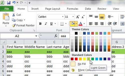
The act of formatting alternating rows with different fill colors is also referred to as “banding.” If you have ever seen an Excel spreadsheet with this effect, then you know how useful it can be in visually organizing your data. However, you might have tried to do it yourself manually, but found that the entire process can be somewhat tedious. Fortunately there is a simple way to automate it that you will find beneficial. Step 1: Open the Excel 2010 spreadsheet to which you want to add your alternating row colors. Step 2: Click the Home tab at the top of the window. Step 3: Click the row heading for the first row to select the entire row, then click the Fill Color button in the font section of the ribbon and choose your first row color.
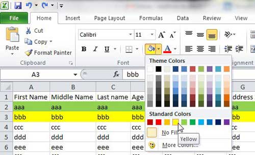
Step 4: Click the row heading for the row underneath that row to select the entire row, click the Fill Color button again, then choose the alternating color.
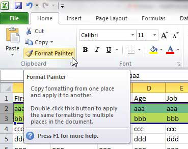
Step 5: Highlight the two rows that you just filled. Step 6: Click the Format Painter button in the Clipboard section of the ribbon.
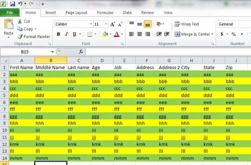
Step 7: Use your mouse to select the rest of the rows to which you want to apply the alternating row colors.
Step 8: Release the mouse button to fill your selected rows with the alternating row colors.
Note that, after you use the Format Painter tool, the rows are not tied to one another in any way. Therefore you can feel free to manually adjust any rows colors that you wish and it will not affect the appearance of the rest of the row colors. After receiving his Bachelor’s and Master’s degrees in Computer Science he spent several years working in IT management for small businesses. However, he now works full time writing content online and creating websites. His main writing topics include iPhones, Microsoft Office, Google Apps, Android, and Photoshop, but he has also written about many other tech topics as well. Read his full bio here.
You may opt out at any time. Read our Privacy Policy
